Simulation and Visualization

This Section describes how open-loop and closed-loop simulations can be realized and how the results can be plotted. Section Solver and Simulator describes the creation and parameterization of a solver as well as the simulation process including the saving of simulation data. Subsequently, Section Using GRAMPC-S with Matlab/Simulink shows how the results can be plotted in Matlab and how GRAMPC-S can be integrated into Simulink using an S-function.

Solver and Simulator

Once the approximation of the stochastic OCP has been selected as described in Section Approximation of the stochastic OCP, a GRAMPC object can be created as a solver using the function

GrampcPtr Solver(ProblemDescriptionPtr problemDescription)

where problemDescription is a shared pointer to the stochastic problem description. Before this solver can be used, the initial states and parameters must be passed to it. Since the representation of states and parameters depends on the used propagation method, these must be calculated by the problem description. All problem descriptions provide the function

void compute_x0_and_p0(DistributionPtr state, DistributionPtr param)

for this purpose. The initial states and parameters can then be accessed by the functions

ctypeRNum* x0()
ctypeRNum* p0()

These can be passed directly to the solver with

solver->setparam_real_vector("x0", problem->x0());
solver->setparam_real_vector("p0", problem->p0());

Next, options and parameters of the solver should be selected. For this purpose, the GRAMPC class provides the member functions

void setopt_real(const char* optName, ctypeRNum optValue)
void setopt_int(const char* optName, ctypeInt optValue)
void setopt_string(const char* optName, const char* optValue)
void setopt_real_vector(const char* optName, ctypeRNum* optValue)
void setopt_int_vector(const char* optName, ctypeInt* optValue)

which call the corresponding GRAMPC functions. For details, please refer to the documentation of GRAMPC. Once the solver has been parameterized, it can be called as follows:

solver->run();

The solution found for the OCP can then be read from the solver object. However, if a closed-loop simulation should be implemented, the actual system behavior must also be simulated, which may deviate from the model of the controller. For this purpose, GRAMPC-S provides the Simulator class, which receives the actual system dynamics, the actual initial states and system parameters. The system can either be simulated without noise, where you can choose between the Euler and Heun method for integration, or simulated with an additive Wiener process, where the Euler-Maruyama method is applied. If the writeDataToFile flag is set, the simulator writes the results of the simulation to text files, which can be plotted in Matlab.

Using GRAMPC-S with Matlab/Simulink

GRAMPC-S is programmed in C++ in order to realize low computation times and to enable implementation on embedded hardware. For reasons of simplicity, however, Matlab is used to plot the results. For this purpose, it is necessary to write the results to text files so they can be read into Matlab afterwards. If a closed-loop simulation is executed, this can be ensured by setting the argument writeDataToFile in the definition of the Simulator object. If no simulator is used because only the OCP is to be solved and the resulting trajectories should be plotted, this can be done with the function

void writeTrajectoriesToFile(GrampcPtr solver, typeInt numberOfStates)

A Matlab script can then be executed to plot the data. The examples/TEMPLATES folder contains three templates:

• plot_simulation: This script plots the results of a closed-loop simulation.

• plot_predicted_trajectories.m: This script plots the obtained solution of the OCP in the current time step for stochastic problem descriptions that represent the states internally in the form of sigma points. These are SigmaPointProblemDescription and MonteCarloProblemDescription.

• plot_predicted_mean_covariance.m: This script plots the found solution of the OCP in the current time step for stochastic problem descriptions that represent the states internally in the form of mean and covariance matrix: These are TaylorProblemDescription, ResamplingProblemDescription, and ResamplingGPProblemDescription.

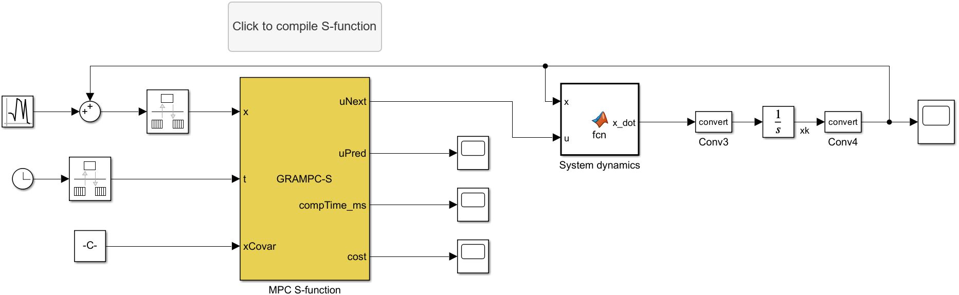
Fig. 1 Simulink model of GRAMPC-S.

GRAMPC-S can also be used in combination with Simulink. Fig. 1 shows the Simulink model of GRAMPC-S, implemented using an S-function. By double-clicking on the button Click to compile S-function, the S-function is compiled and can be used for the simulation in Simulink. Before compiling, make sure that the folder containing the Simulink model is open in Matlab. The Simulink model shown in Fig. 1 is located in the folder examples/inverted_pendulum and is designed for the example of an inverted pendulum. The S-function is implemented in the file grampc_s_Sfct.cpp in the same folder. The S-function must be adapted accordingly for use with other systems. The model parameters, such as sampling time, initial states, etc., are set in the initFct callback of the Simulink model, which can be found in Modeling → Model Properties → Callbacks.